Prostitution in the US: Price

How much US sex workers charge depends on a variety of factors

Note: This is the fourth of several installments. Part 1 explored the dataset, part 2 looked at the ethnicity of sex workers, part 3 looked at the services performed and how this correlates to ethnicity, part 4 (this part) looks at the economic side of things, and how fees correlate to ethnicity, services and looks of sex workers.

We are ready to look at the cost of services, but before we go there, let’s look at the looks. Not all providers are created equal and TER reviews certainly reflect that.

Hey, Sexy Lady!

Our dataset also offers assessments of providers’ looks. Rating is often missing for newer providers. We have Stars and looks. We will consolidate those values into categorical variables, to make it easier for us to create diagrams and visualize the data.

We have Stars, Rating and Looks in our data.

Many providers have not accrued enough reviews to get their stars assigned. Those who do break down like this:

We are doing something similar for Rating and Looks:

Distribution of Rating

Distribution of Looks

Stars, looks and ratings will be interesting to correlate with price, once we have that data.

Time to talk money

The dataset doesn’t offer a clear straight figure about the cost of the offered service. Currency is one issue. Outside of the US, reviewers have provided prices in two or more currencies (Hong Kong, for example, uses USD, local dollars and Chinese Yuans). But there’s a bigger problem. Some reviews carry multiple reports about the prices, some referring to fraction of an hour, some to multiple hours or even days.

For this reason, we first need to create a normalized price, i.e. a figure that allows us to compare, you guessed it, apple to apple.

In practice:

• currency is first normalized (also keeping country of provider into account whenever necessary, as many countries call their currency Dollars and use the $ symbol).
• if a provider has a single entry and that entry refers to one-hour service, then we are done (other entries are discarded).
• if provider has multiple entries that refer to one hour, the average of those entries is taken (other entries are discarded).
• if provider has no “one hours” but has a fraction or a multiple of one hour, hourly price is calculated through proportional adjustement.
• if provider has no “one hours” but has multiple fractions or a multiples of one hour, hourly price is calculated for each item and an average one-hour rate is calculated.

Note: If the calculated amounts is less than a reasonable threshold (higher for western countries), the result will be float("NaN") (i.e. the equivalent of a missing piece of data) as we are probably looking at a bogus entry. Those records will be discarded for the purposes of the relevant data visualizations.

The normalized price is added as a brand new ‘Hourly Price’ column.

The following code snippets are provided to let data people get a glimpse of the ETL that was performed to make the data uniform.

Converting currencies was a bitch, but it was key to enable apple to apple comparisons

#time to create the new column
frame["Hourly Price"] = frame.apply(lambda row: get_avg_price(row.name, row['Country'],row['City'], row['Price-1'], row['Price-2'],row['Price-3'],row['Price-4'],                  row['Price-5'], row['Price-6'],row['Price-7'],row['Price-8'],  row['Time-1'], row['Time-2'],row['Time-3'], row['Time-4'],
row['Time-5'], row['Time-6'],row['Time-7'],row['Time-8']), axis=1)

Normalizing currencies was a bitch, but we can compare costs across countries, states and cities now:

mycountries = ['USA','Canada','Germany','Mexico','Argentina','Brazil', 'United Kingdom','France','Spain','Switzerland', 'Dominican Republic',
'Philippines','Colombia','Russia','Hong Kong']
 
frame[frame.Country.isin(mycountries)].groupby(['Country']).agg({'Hourly Price':['mean']}).plot(kind="barh", grid=True, figsize=(10,10));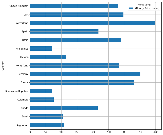

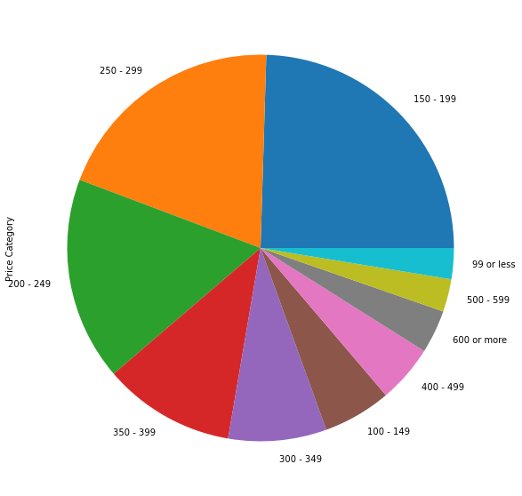
Average prices (in USD) in different countries. Switzerland is expensive. Dominican Republic is cheap.

Let’s zoom in on the US “market” and see how things break down:

cut_labels_stars = ['99 or less','100 - 149', '150 - 199', '200 - 249', '250 - 299','300 - 349', '350 - 399', '400 - 499', '500 - 599','600 or more']
cut_bins = [0,100, 150, 200, 250, 300, 350 , 400, 500, 600, 200000]
frame['Price Category'] = pd.cut(frame['Hourly Price'], bins=cut_bins, labels=cut_labels_stars)
frame[frame.Country=="USA"]['Price Category'].value_counts(normalize=True).plot(kind="pie")

The overwhelming majority of reviewers pay between 150 and 350 to get service in the US

How do price and looks correlate? Unsurprisingly, providers that got the looks also command conspicuously higher prices.

frame[frame.Country == "USA"][['Looks Category','Hourly Price']].groupby("Looks Category").mean().plot(kind="barh", grid=True);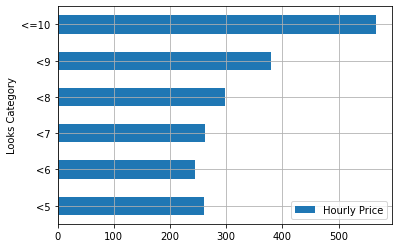

Extremely attractive providers (looks higher than 9 out of 10) command higher prices for their services

Let’s see if our data tells us where the best looking dolls are hanging out (spoiler alert: San Francisco, LA and NYC.)

The prettiest providers hang out in San Francisco, LA and NYC

You got the looks but have you got the touch?

Stars vs. Price: lots of stars = lots of money.

frame[frame.Country == "USA"][['Stars Category','Hourly Price']].groupby("Stars Category").mean().plot(kind="barh", grid=True);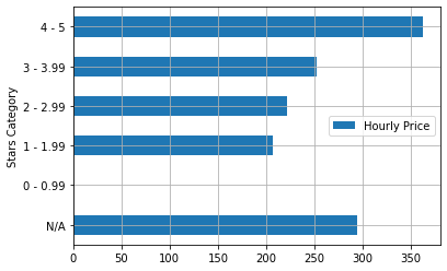

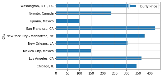
The prettiest providers (4 stars or more) make more money per hour

Average prices in main US cities (spoiler alert: San Francisco, New York and LA are the most expensive).

keycities = ["New York City - Manhattan, NY", "Los Angeles, CA", "San Francisco, CA", "Chicago, IL", "Washington, D.C., DC", 
             "Mexico City, Mexico", "New Orleans, LA", "Toronto, Canada", "Tijuana, Mexico"]
frame[frame.City.isin(keycities)][['City','Hourly Price']].groupby("City").mean().plot(kind="barh", grid=True);

Unsurprisingly, San Francisco, LA and NYC are also the place where services are the most expensive

Ethnicity vs. Cost: is there a correlation between ethnicity and the price that an escort either requests or can request? You bet. White chicks and latinas make more money than African American and Asian sex workers. About $50 more.

frame[frame.Country == "USA"][['EthnicityNormalized','Hourly Price']].groupby("EthnicityNormalized").mean().plot(kind="barh",grid=True);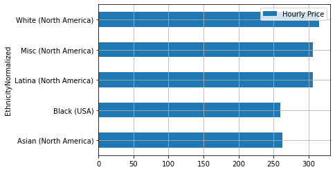

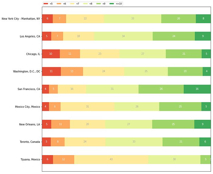
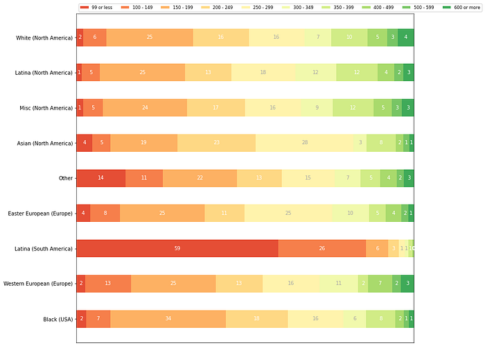
US-based Black and Asian workers seem to make, on average, $60 less per hour as compared to white providers

This diagram compares price categories across ethnicities side by side. I threw in LATAM providers for perspective:

A wider look that also involves other parts of the world shows that South and Central America means vastly cheaper hourly price

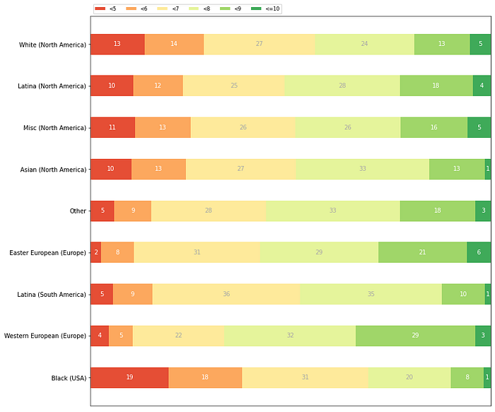
Is there a correlation between ethnicity and perceived attractiveness. The data suggests so. African American providers as perceived as slightly less pretty than other ethnicities.

Black providers are generally considered less attractive than other ethnicities

Up the Butt

Anal Sex vs. Price: if you guessed that a correlation is there, you guessed right, it correlates.

Note: YMMV stands for Your Mileage May Vary, meaning that provider will agree to anal sex, albeit she’s not a “greek” natural.

frame[frame.Country == "USA"][['Anal','Hourly Price']].groupby("Anal").mean().plot(kind="barh", grid=True);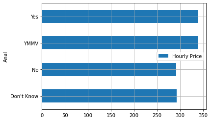

US providers that either provide anal sex or at least try get on average $50 more per hour

My milkshake is better than yours

Ejaculate in the Mouth vs. Price: yes, this also correlates.

US providers that let clients come in their mouths (CIM) make an additional $20 per hour on average. If they swallow, that’s an extra $50 (i.e. $70 per hour totally)

frame[frame.Country == "USA"][['Cum In Mouth','Hourly Price']].groupby("Cum In Mouth").mean().plot(kind="barh", grid=True);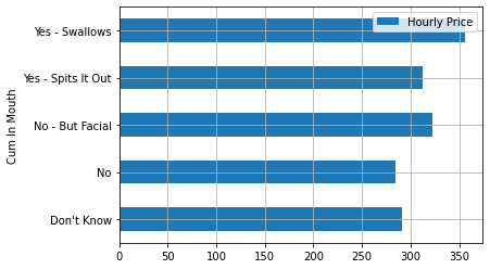

CIM = $20 per hour on average. Swallowers make an additional $50 (i.e. $70 per hour totally)

Not everyone’s cup of tea

Squirt vs. Price: not everyone’s cup of tea, I guess. But still popular enough that escorts with this particular ability command a higher price for the service.

frame[frame.Country == "USA"][['Squirt','Hourly Price']].groupby("Squirt").mean().plot(kind="barh", grid=True);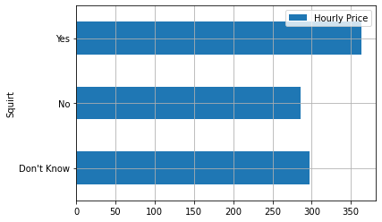

Squirting commands an extra $80 per hour

Harder, Harder!

S&M vs. Price. Also correlates of course.

frame[frame.Country == "USA"][['S&M','Hourly Price']].groupby("S&M").mean().plot(kind="barh", grid=True);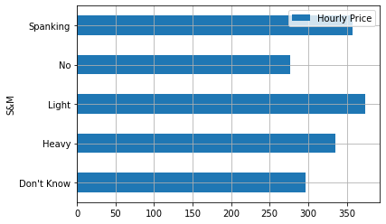

Different levels of S&M services may make up to an extra $100 for adventurous providers

The postman always rings twice

Multiple Shots on Goal vs. Price: some escorts let their clients come more than once per session, a service called MSOG for Multiple Shots on Target.

frame[frame.Country == "USA"][['Multiple Pops Allowed','Hourly Price']].groupby("Multiple Pops Allowed").mean().plot(kind="barh", grid=True);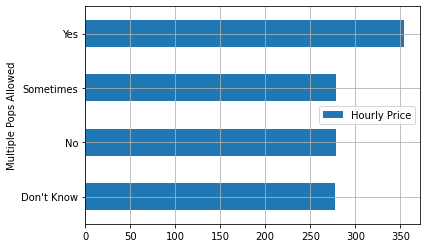

Providers who let the customers come twice make an additional $80 per hour

On the way to stardom

Pornstars command a much higher price. I guess the guy is in a hurry to… go tell his friends at the pub (old Australian joke I once heard).

frame[frame.Country == "USA"][['Porn Star','Hourly Price']].groupby("Porn Star").mean().plot(kind="barh", grid=True);

Porn stars can make a staggering additional $150 per hour on average

Grab her by the pussy

Touch Pussy vs. Price: Donald is not the only one who wants to touch it. Many dudes will pay handsomely for the privilege.

frame[frame.Country == "USA"][['Touch Pussy','Hourly Price']].groupby("Touch Pussy").mean().plot(kind="barh", grid=True);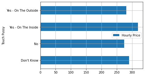

Access to vagina grants an additional $60 on average

That’s it for now

This was for me a project to test my abilities as a data journalist. I had not planned to disclose my findings, but once I managed to collect the data and analyze it, it seemed a waste not to share it, albeit I am sure many feminists will hate me for this.

If you like the articles, please clap.

If you have questions about the data, please add them to comments. Time permitting, I may answer them. Thank you.